40 excel 2013 data labels

Custom Data Labels with Colors and Symbols in Excel Charts - [How To] Step 4: Select the data in column C and hit Ctrl+1 to invoke format cell dialogue box. From left click custom and have your cursor in the type field and follow these steps: Press and Hold ALT key on the keyboard and on the Numpad hit 3 and 0 keys. Let go the ALT key and you will see that upward arrow is inserted. Adding rich data labels to charts in Excel 2013 - Microsoft 365 Blog You can do this by adjusting the zoom control on the bottom right corner of Excel's chrome. Then, select the value in the data label and hit the right-arrow key on your keyboard. The story behind the data in our example is that the temperature increased significantly on Wednesday and that appeared to help drive up business at the lemonade stand.

Excel Data Labels - Value from Cells 4. Sign in to vote. I created a chart and linked the data labels to a series of cells, as 2013 allows in Value From Cells option. I pre-select e.g. 100 data rows even though it initially contains values in 10 of them. When I reopen the workbook and add x and y value and a new label (where I left empty cells to do so) that data point 'icon ...

Excel 2013 data labels

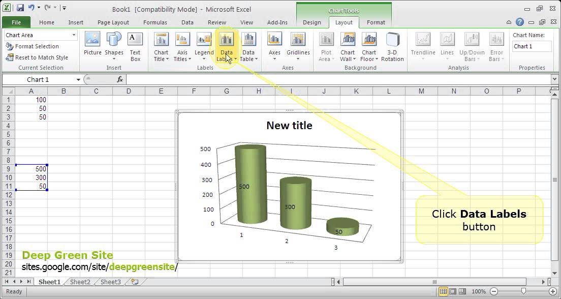
How to add data labels from different column in an Excel chart? Right click the data series in the chart, and select Add Data Labels > Add Data Labels from the context menu to add data labels. 2. Click any data label to select all data labels, and then click the specified data label to select it only in the chart. 3. Change the format of data labels in a chart To get there, after adding your data labels, select the data label to format, and then click Chart Elements > Data Labels > More Options. To go to the appropriate area, click one of the four icons ( Fill & Line, Effects, Size & Properties ( Layout & Properties in Outlook or Word), or Label Options) shown here. Adding Data Labels to Your Chart (Microsoft Excel) To add data labels in Excel 2013 or Excel 2016, follow these steps: Activate the chart by clicking on it, if necessary. Make sure the Design tab of the ribbon is displayed. (This will appear when the chart is selected.) Click the Add Chart Element drop-down list. Select the Data Labels tool.

Excel 2013 data labels. Tip - Adding rich data labels to charts in Excel 2013 You can do this by adjusting the zoom control on the bottom right corner of Excel's chrome. Then, select the value in the data label and hit the right-arrow key on your keyboard. The story behind the data in our example is that the temperature increased significantly on Wednesday and that appeared to help drive up business at the lemonade stand. How to Print Labels from Excel - Lifewire Choose Start Mail Merge > Labels . Choose the brand in the Label Vendors box and then choose the product number, which is listed on the label package. You can also select New Label if you want to enter custom label dimensions. Click OK when you are ready to proceed. Connect the Worksheet to the Labels Format Data Labels in Excel- Instructions - TeachUcomp, Inc. To format data labels in Excel, choose the set of data labels to format. To do this, click the "Format" tab within the "Chart Tools" contextual tab in the Ribbon. Then select the data labels to format from the "Chart Elements" drop-down in the "Current Selection" button group. Excel 2013 Tutorial Formatting Data Labels Microsoft Training ... - YouTube FREE Course! Click: about formatting data labels in Microsoft Excel at . A clip from Mastering Excel M...

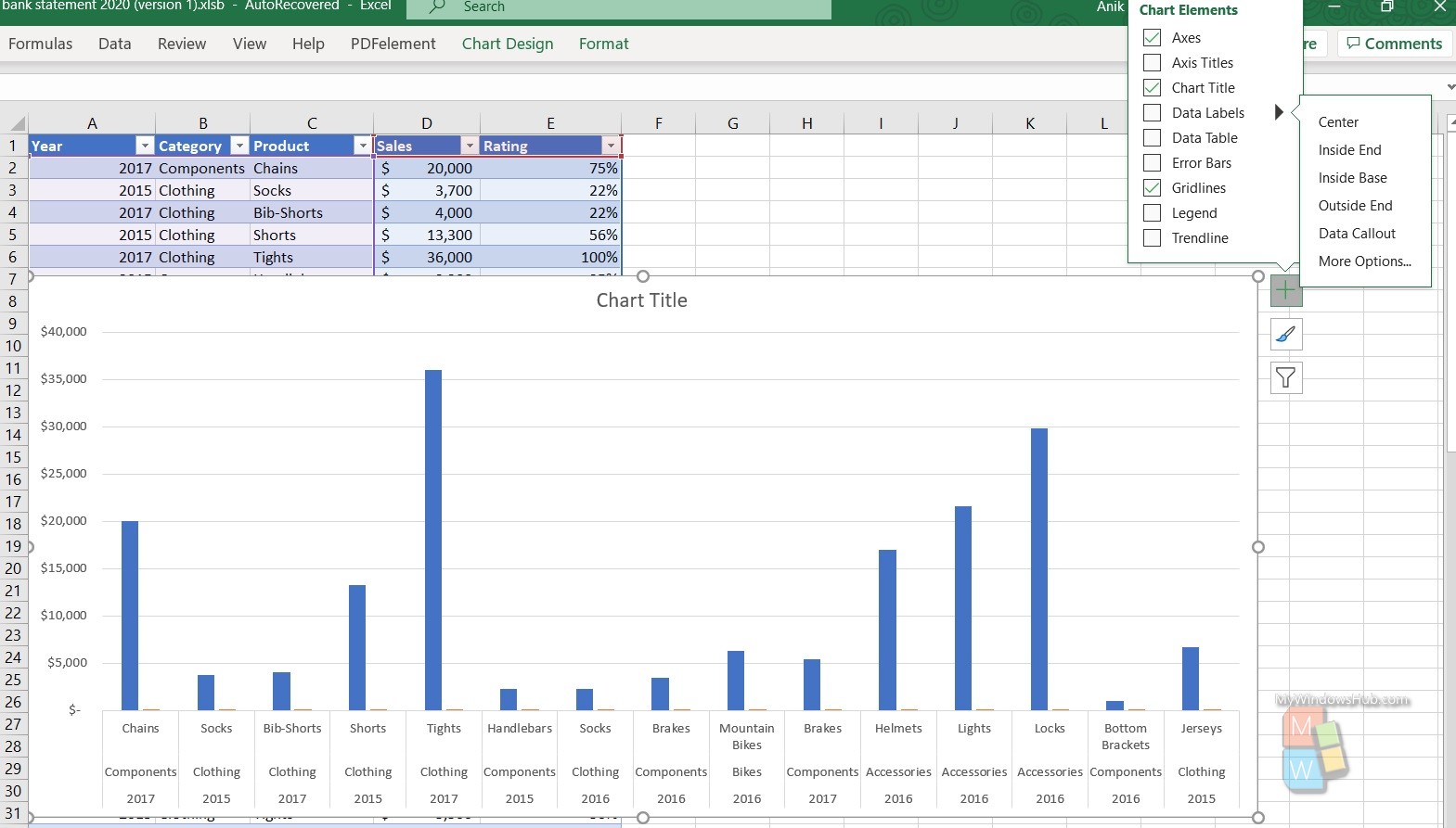
How to Add Data Labels in Excel - Excelchat | Excelchat In Excel 2013 and the later versions we need to do the followings; Click anywhere in the chart area to display the Chart Elements button Figure 5. Chart Elements Button Click the Chart Elements button > Select the Data Labels, then click the Arrow to choose the data labels position. Figure 6. How to Add Data Labels in Excel 2013 Figure 7. How to Customize Chart Elements in Excel 2013 - dummies To add data labels to your selected chart and position them, click the Chart Elements button next to the chart and then select the Data Labels check box before you select one of the following options on its continuation menu: Center to position the data labels in the middle of each data point. Inside End to position the data labels inside each ... Excel 2013 Graphs automatically aligning data labels to end of bar Posts: 14. Excel 2013 Graphs automatically aligning data labels to end of bar. Hi. In Excel 2013 I am wanting to align the data labels in a graph automatically to be at the end of the bar (in a bar graph obviously). I know how to move them manually, but I remember there used to be a way to make it move them all automatically. mgconsulting.wordpress.com › 2013/12/09 › add-a-dataAdd a Data Callout Label to Charts in Excel 2013 In the upper right corner, next to your chart, click the Chart Elements button (plus sign), and then click Data Labels. A right pointing arrow will appear, click on this arrow to view the submenu. Select Data Callout. Once the Data Callout Labels have been added, you can re-position them by clicking on their borders and dragging to a new position.

› excel_barcode › data_encodingFree Download Excel 2016/2013 QR Code Generator. No barcode ... Create EAN-128 in Excel 2016/2013/2010/2007. Not barcode EAN-128/GS1-128 font, excel macro. Full demo source code free download. Excel 2016/2013 Data Matrix generator add-in. Full demo source code free download. Not barcode Data Matrix font, excel formula. Not barcode font. Generate UPC-A in excel spreadsheet using barcode Excel add-in. No need ... Values From Cell: Missing Data Labels Option in Excel 2013? When a chart created in 2013 using the "Values from Cell" data label option is opened with any earlier version of Excel, the data labels will show as " [CELLRANGE]". If you want to ensure that data labels survive different generations of Excel, you need to revert to the old technique: Insert data labels Edit each individual data label Add or remove data labels in a chart - support.microsoft.com To label one data point, after clicking the series, click that data point. In the upper right corner, next to the chart, click Add Chart Element > Data Labels. To change the location, click the arrow, and choose an option. If you want to show your data label inside a text bubble shape, click Data Callout. How to Add Data Labels to your Excel Chart in Excel 2013 Data labels show the values next to the corresponding chart element, for instance a percentage next to a piece from a pie chart, or a total value next to a column in a column chart. You can choose...

How to Make Labels from Excel

Excel Tips n Tricks -Tip 8 (Applying Chart Data Labels From a Range in ... It will popup a Range Selector dialog box. Select the Column containing the text for the chart data and click "OK". Remember that the text should belong to the cell adjacent to the label data. Picture 7. 6. All done, just hit Enter or click "Ok" and you have your chart decorated with the text for data labels like this:

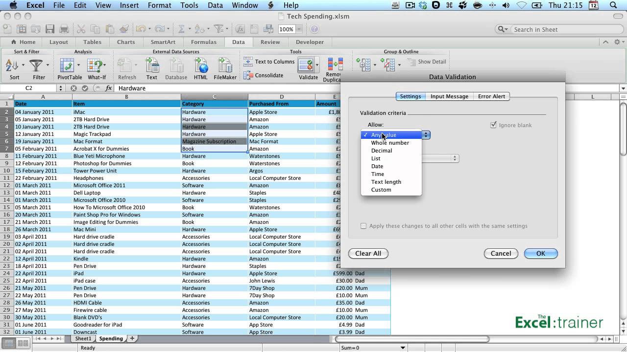
Excel : Data Validation & Drop Down Lists - YouTube

Excel 2013 Chart Labels don't appear properly - Microsoft Community You've stumbled on a big problem - Excel 2013 lets you edit data labels directly, but this feature (rich text data labels) is not backwards-compatible and there's no way to turn it off. It's great to be able to modify the text of labels, or direct them to get contents from a worksheet cell.

Example: Charts with Data Tools — XlsxWriter Documentation

How to hide zero data labels in chart in Excel? - ExtendOffice Note: In Excel 2013, you can right click the any data label and select Format Data Labels to open the Format Data Labels pane; then click Number to expand its option; next click the Category box and select the Custom from the drop down list, and type #"" into the Format Code text box, and click the Add button.

Format Data Labels in Excel- Instructions | Microsoft excel, Microsoft, Bar chart

Values From Cell: Missing Data Labels Option in Excel 2013? A couple articles refer to formatting data labels and values to have it pull what you want. I have a feeling they used a 3rd party ad-in like tech-cell or some such and because I don't have the add in its not happy. Im following the blog reference here: Adding rich data labels to charts in Excel 2013 - Office Blogs

35 Label Of Microsoft Excel - Label Design Ideas 2020

› charts › dynamic-chart-dataCreate Dynamic Chart Data Labels with Slicers - Excel Campus Feb 10, 2016 · Typically a chart will display data labels based on the underlying source data for the chart. In Excel 2013 a new feature called “Value from Cells” was introduced. This feature allows us to specify the a range that we want to use for the labels. Since our data labels will change between a currency ($) and percentage (%) formats, we need a ...

MS Excel 2010 / How to remove data labels from the chart - YouTube

Quick Tip: Excel 2013 offers flexible data labels | TechRepublic right-click and choose Insert Data Label Field. In the next dialog, select [Cell] Choose Cell. When Excel displays the source dialog, click the cell that contains the MIN () function, and click OK....

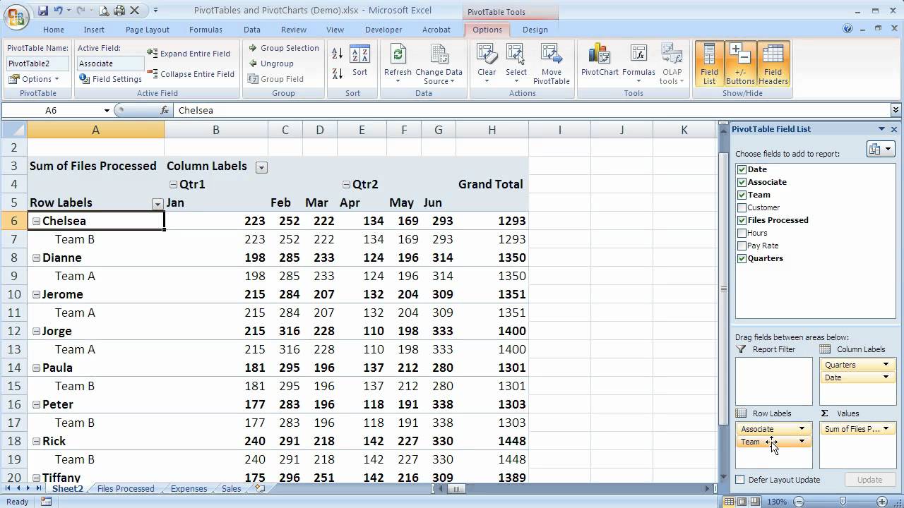
How to group row labels in Excel 2007 PivotTables (Excel 07-104) - YouTube

data labels in chart - excel 2013 | MrExcel Message Board Hi I have 3 data labels in column chart. I changed the shape of these labels to Oval Callout. if I select one of them to format, then they will be all selected as well. Which is good and understandable. But how can I move them all at same time. Now when I click on one of them then they will all...

Format Number Options for Chart Data Labels in Excel 2011 for Mac

› excel_barcodeExcel Barcode Generator Add-in: Create Barcodes in Excel 2019 ... Office Excel Barcode Encoder Add-In is a reliable, efficient and convenient barcode generator for Microsoft Excel 2016/2013/2010/2007, which is designed for office users to embed most popular barcodes into Excel workbooks. It is widely applied in many industries.

What's New With Excel 2016? - Microsoft Office Tutorials | SEO Tips

chandoo.org › wp › change-data-labels-in-chartsHow to Change Excel Chart Data Labels to Custom Values? May 05, 2010 · Now, click on any data label. This will select “all” data labels. Now click once again. At this point excel will select only one data label. Go to Formula bar, press = and point to the cell where the data label for that chart data point is defined. Repeat the process for all other data labels, one after another. See the screencast.

How To Show Or Hide Data Labels On MS Excel? | My Windows Hub

support.microsoft.com › en-us › officeTutorial: Import Data into Excel, and Create a Data Model However, the same data modeling and Power Pivot features introduced in Excel 2013 also apply to Excel 2016. In these tutorials you learn how to import and explore data in Excel, build and refine a data model using Power Pivot, and create interactive reports with Power View that you can publish, protect, and share.

Format Number Options for Chart Data Labels in Excel 2011 for Mac

Excel 2013 charting--can't display over 1000 labels In Excel 2013, only 1 label is displayed with the message that it can't display over 1000 labels. In 2007 and 2010, the labels are displayed perfectly. According to a co-worker that has taken an Excel class, the instructor was aware of this bug in 2013, however, I have only been able to find one other instance of this problem on the web.

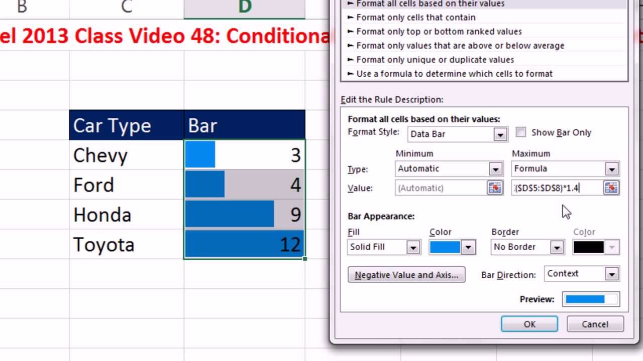
Highline Excel 2013 Class Video 48: Conditional Formatting: Bar Chart with Data Labels - YouTube

Excel 2013 Project Timeline - colour coding data labels I've created a timeline using the Excel 2013 Project Timeline template. Is there any way to colour code the Milestone data fonts in the Project Details Table so that it automatically updates the Data Labels on the timeline to the same colour? Simply changing the font colour in the table doesn't do it.

35 What Is Data Label In Excel - Labels For You

Creating a chart with dynamic labels - Microsoft Excel 2013 Excel 2013 365 2016. This tip shows how to create dynamically updated chart labels that depend on value or other cells. ... For all labels: on the Format Data Labels task pane, in the Label Options, in the Label Contains group, check Value From Cells and then choose cells:

How to Create Multi-Category Chart in Excel - Excel Board

Excel 2013 Chart label not displaying At the moment I have data labels with percentages. All other labels display, of which there are 7. I found a solution that fixes the problem each time it arises and that is to select Chart Tools/Format/Series 1 data labels and then Format Selection. When I then select any data label, I click on "Clone Current Label" and the missing label ...

One-Way ANOVA with Microsoft Excel | Pharmacy Math Made Simple!

› excel › how-to-add-total-dataHow to Add Total Data Labels to the Excel Stacked Bar Chart Apr 03, 2013 · Step 4: Right click your new line chart and select “Add Data Labels” Step 5: Right click your new data labels and format them so that their label position is “Above”; also make the labels bold and increase the font size. Step 6: Right click the line, select “Format Data Series”; in the Line Color menu, select “No line”

Excel Bar Charts - Clustered, Stacked - Template - Automate Excel

Custom Chart Labels Using Excel 2013 | MyExcelOnline View the Benchmark Chart using Excel 2013. DOWNLOAD EXCEL WORKBOOK. STEP 1: We added a % Variance column in our data and inserted symbols to show a negative and positive variance. ** You can see the tutorial of how this is done here **. STEP 2: In our graph we need to select the Sales chart and Right Click and choose Add Data Labels.

How to Create and Label a Pie Chart in Excel 2013 : 8 Steps - Instructables

Adding Data Labels to Your Chart (Microsoft Excel) To add data labels in Excel 2013 or Excel 2016, follow these steps: Activate the chart by clicking on it, if necessary. Make sure the Design tab of the ribbon is displayed. (This will appear when the chart is selected.) Click the Add Chart Element drop-down list. Select the Data Labels tool.

Share :