41 how to show data labels in excel

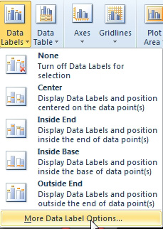
Add data labels and callouts to charts in Excel 365 - EasyTweaks.com Step #1: After generating the chart in Excel, right-click anywhere within the chart and select Add labels . Note that you can also select the very handy option of Adding data Callouts. Excel 2010: Show Data Labels In Chart - AddictiveTips To enable data labels in chart, select the chart and head over to Chart Tools Layout tab, from Labels group, under Data Labels options, select a position. It will show Data labels at specified position. Likewise, from Data Labels pull-down menu, you can change the position of data labels and access other advance options. ← Splash Lite ...

Excel charts: how to move data labels to legend - Microsoft Tech Community @Matt_Fischer-Daly . You can't do that, but you can show a data table below the chart instead of data labels: Click anywhere on the chart. On the Design tab of the ribbon (under Chart Tools), in the Chart Layouts group, click Add Chart Element > Data Table > With Legend Keys (or No Legend Keys if you prefer)

How to show data labels in excel

how to add data labels into Excel graphs - storytelling with data There are a few different techniques we could use to create labels that look like this. Option 1: The "brute force" technique. The data labels for the two lines are not, technically, "data labels" at all. A text box was added to this graph, and then the numbers and category labels were simply typed in manually. How to add data labels from different column in an Excel chart? Click any data label to select all data labels, and then click the specified data label to select it only in the chart. 3. Go to the formula bar, type =, select the corresponding cell in the different column, and press the Enter key. See screenshot: 4. Repeat the above 2 - 3 steps to add data labels from the different column for other data points. How to Add Data Labels to an Excel 2010 Chart - dummies Use the following steps to add data labels to series in a chart: Click anywhere on the chart that you want to modify. On the Chart Tools Layout tab, click the Data Labels button in the Labels group. A menu of data label placement options appears: None: The default choice; it means you don't want to display data labels. Center to position the ...

How to show data labels in excel. How To Create Labels In Excel - host RS Column names in your spreadsheet match the field names you want to insert in your labels. Right click the data series in the chart, and select add data labels > add data labels from the context menu to add data labels. In the mailings tab of word, select the finish & merge option and choose edit individual documents from the menu. How to find, highlight and label a data point in Excel scatter plot Select the Data Labels box and choose where to position the label. By default, Excel shows one numeric value for the label, y value in our case. To display both x and y values, right-click the label, click Format Data Labels…, select the X Value and Y value boxes, and set the Separator of your choosing: Label the data point by name Format Data Labels in Excel- Instructions - TeachUcomp, Inc. To do this, click the "Format" tab within the "Chart Tools" contextual tab in the Ribbon. Then select the data labels to format from the "Chart Elements" drop-down in the "Current Selection" button group. Then click the "Format Selection" button that appears below the drop-down menu in the same area. Add a DATA LABEL to ONE POINT on a chart in Excel Click on the chart line to add the data point to. All the data points will be highlighted. Click again on the single point that you want to add a data label to. Right-click and select ' Add data label ' This is the key step! Right-click again on the data point itself (not the label) and select ' Format data label '.

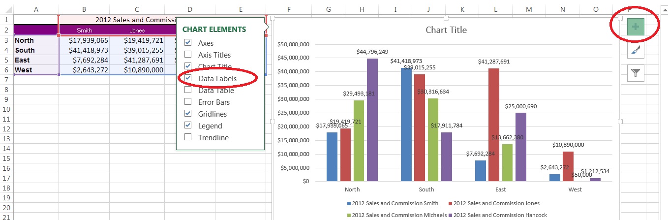
Excel tutorial: How to use data labels Generally, the easiest way to show data labels to use the chart elements menu. When you check the box, you'll see data labels appear in the chart. If you have more than one data series, you can select a series first, then turn on data labels for that series only. You can even select a single bar, and show just one data label. How to show data label in "percentage" instead of - Microsoft Community Select Format Data Labels Select Number in the left column Select Percentage in the popup options In the Format code field set the number of decimal places required and click Add. (Or if the table data in in percentage format then you can select Link to source.) Click OK Regards, OssieMac Report abuse 8 people found this reply helpful · How to Add Two Data Labels in Excel Chart (with Easy Steps) You can easily show two parameters in the data label. For instance, you can show the number of units as well as categories in the data label. To do so, Select the data labels. Then right-click your mouse to bring the menu. Format Data Labels side-bar will appear. You will see many options available there. Check Category Name. Custom Chart Data Labels In Excel With Formulas Follow the steps below to create the custom data labels. Select the chart label you want to change. In the formula-bar hit = (equals), select the cell reference containing your chart label's data. In this case, the first label is in cell E2. Finally, repeat for all your chart laebls.

Display every "n" th data label in graphs - Microsoft Community With this tool you can assign a range of cells to be the labels for chart series, instead of the Excel defaults. Using a formula, you can have a text show up in every nth cell and then use that range with the XY Chart Labeler to display as the series label. If the full chart labels are in column A, starting in cell A1, then you can use this ... Add or remove data labels in a chart - support.microsoft.com Click Label Options and under Label Contains, select the Values From Cells checkbox. When the Data Label Range dialog box appears, go back to the spreadsheet and select the range for which you want the cell values to display as data labels. When you do that, the selected range will appear in the Data Label Range dialog box. Then click OK. How to Add Data Labels in Excel - Excelchat | Excelchat In Excel 2013 and the later versions we need to do the followings; Click anywhere in the chart area to display the Chart Elements button Figure 5. Chart Elements Button Click the Chart Elements button > Select the Data Labels, then click the Arrow to choose the data labels position. Figure 6. How to Add Data Labels in Excel 2013 Figure 7. How to hide zero data labels in chart in Excel? - ExtendOffice In the Format Data Labelsdialog, Click Numberin left pane, then selectCustom from the Categorylist box, and type #""into the Format Codetext box, and click Addbutton to add it to Typelist box. See screenshot: 3. Click Closebutton to close the dialog. Then you can see all zero data labels are hidden.

Excel: Formatting Charts in Excel 2010 with Layout - Excel Articles

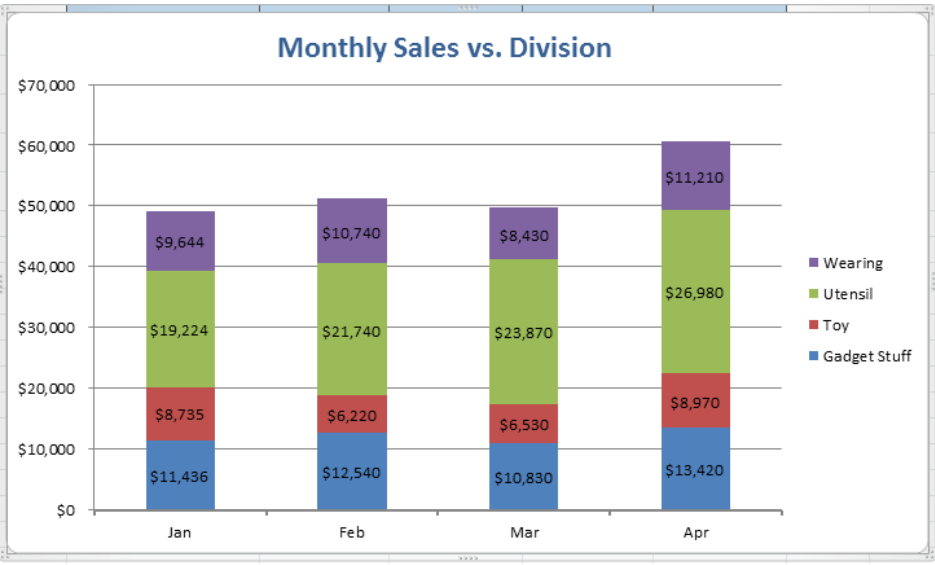
How to Add Labels to Show Totals in Stacked Column Charts in Excel In the chart, right-click the "Total" series and then, on the shortcut menu, select Add Data Labels. 9. Next, select the labels and then, in the Format Data Labels pane, under Label Options, set the Label Position to Above. 10. While the labels are still selected set their font to Bold. 11.

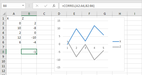
Correlation in Excel - Easy Excel Tutorial

How to create Custom Data Labels in Excel Charts Add default data labels. Click on each unwanted label (using slow double click) and delete it. Select each item where you want the custom label one at a time. Press F2 to move focus to the Formula editing box. Type the equal to sign. Now click on the cell which contains the appropriate label. Press ENTER.

Excel: Grouping pivot table entries

Change the format of data labels in a chart To get there, after adding your data labels, select the data label to format, and then click Chart Elements > Data Labels > More Options. To go to the appropriate area, click one of the four icons ( Fill & Line, Effects, Size & Properties ( Layout & Properties in Outlook or Word), or Label Options) shown here.

Excel Charts: Creating Custom Data Labels - YouTube

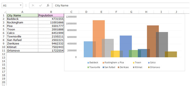
How to Add Labels to Scatterplot Points in Excel - Statology Step 3: Add Labels to Points. Next, click anywhere on the chart until a green plus (+) sign appears in the top right corner. Then click Data Labels, then click More Options…. In the Format Data Labels window that appears on the right of the screen, uncheck the box next to Y Value and check the box next to Value From Cells.

410 How to display percentage labels in pie chart in Excel 2016 - YouTube

How to Print Labels From Excel - Lifewire To label legends in Excel, select a blank area of the chart. In the upper-right, select the Plus ( +) > check the Legend checkbox. Then, select the cell containing the legend and enter a new name. How do I label a series in Excel? To label a series in Excel, right-click the chart with data series > Select Data.

Displaying Numbers in Thousands in a Chart in Microsoft Excel

How to use data labels in a chart - YouTube Excel charts have a flexible system to display values called "data labels". Data labels are a classic example a "simple" Excel feature with a huge range of o...

microsoft excel - Adding data label only to the last value - Super User

Data label name appear on hover - Excel Help Forum For a new thread (1st post), scroll to Manage Attachments, otherwise scroll down to GO ADVANCED, click, and then scroll down to MANAGE ATTACHMENTS and click again. Now follow the instructions at the top of that screen. New Notice for experts and gurus:

Enable or Disable Excel Data Labels at the click of a button - How To - PakAccountants.com

How to Show Pie Chart Data Labels in Percentage in Excel Then select Format Data Labels from the appeared context menu, soon the Format Data Labels field will appear. Or you can double click on any data label to open the Format Data Labels field directly. Then just mark the Percentage option from the Label Options. Then you will get the data labels like the image below.

Line Chart in Excel - Easy Excel Tutorial

How to Change Excel Chart Data Labels to Custom Values? Now, click on any data label. This will select "all" data labels. Now click once again. At this point excel will select only one data label. Go to Formula bar, press = and point to the cell where the data label for that chart data point is defined. Repeat the process for all other data labels, one after another. See the screencast. Points to note:

Bubble Chart: How to create it in excel - DataWitzz

How to Add Data Labels to an Excel 2010 Chart - dummies Use the following steps to add data labels to series in a chart: Click anywhere on the chart that you want to modify. On the Chart Tools Layout tab, click the Data Labels button in the Labels group. A menu of data label placement options appears: None: The default choice; it means you don't want to display data labels. Center to position the ...

SQL Workbench/J User's Manual SQLWorkbench

How to add data labels from different column in an Excel chart? Click any data label to select all data labels, and then click the specified data label to select it only in the chart. 3. Go to the formula bar, type =, select the corresponding cell in the different column, and press the Enter key. See screenshot: 4. Repeat the above 2 - 3 steps to add data labels from the different column for other data points.