42 how to show labels in excel chart
How to create a chart with both percentage and value in … 1. Click Kutools > Charts > Category Comparison > Stacked Chart with Percentage, see screenshot: 2. In the Stacked column chart with percentage dialog box, specify the data range, axis labels and legend series from the original data range separately, see screenshot: 3. How to use data labels in a chart - YouTube Excel charts have a flexible system to display values called "data labels". Data labels are a classic example a "simple" Excel feature with a huge range of o...
Find, label and highlight a certain data point in Excel ... Select the Data Labels box and choose where to position the label. By default, Excel shows one numeric value for the label, y value in our case. To display both x and y values, right-click the label, click Format Data Labels…, select the X Value and Y value boxes, and set the Separator of your choosing: Label the data point by name
How to show labels in excel chart
How to Create a Bar Chart With Labels Above Bars in Excel In the Format Data Labels pane, under Label Options selected, set the Label Position to Inside Base. 10. Then, under Label Contains, check the Category Name option and uncheck the Value and Show Leader Lines options. 11. Next, while the labels are still selected, click on Text Options, and then click on the Textbox icon. 12. Excel tutorial: How to use data labels Generally, the easiest way to show data labels to use the chart elements menu. When you check the box, you'll see data labels appear in the chart. If you have more than one data series, you can select a series first, then turn on data labels for that series only. You can even select a single bar, and show just one data label. Custom Chart Data Labels In Excel With Formulas Follow the steps below to create the custom data labels. Select the chart label you want to change. In the formula-bar hit = (equals), select the cell reference containing your chart label's data. In this case, the first label is in cell E2. Finally, repeat for all your chart laebls.
How to show labels in excel chart. How to Change Excel Chart Data Labels to Custom Values? This will select "all" data labels. Now click once again. At this point excel will select only one data label. Go to Formula bar, press = and point to the cell where the data label for that chart data point is defined. Repeat the process for all other data labels, one after another. See the screencast. Points to note: How to rotate axis labels in chart in Excel? 1. Right click at the axis you want to rotate its labels, select Format Axis from the context menu. See screenshot: 2. In the Format Axis dialog, click Alignment tab and go to the Text Layout section to select the direction you need from the list box of Text direction. See screenshot: 3. Close the dialog, then you can see the axis labels are rotated. Format Data Labels in Excel- Instructions - TeachUcomp, Inc. To do this, click the "Format" tab within the "Chart Tools" contextual tab in the Ribbon. Then select the data labels to format from the "Chart Elements" drop-down in the "Current Selection" button group. Then click the "Format Selection" button that appears below the drop-down menu in the same area. support.microsoft.com › en-us › officeAdd or remove data labels in a chart Click Label Options and under Label Contains, select the Values From Cells checkbox. When the Data Label Range dialog box appears, go back to the spreadsheet and select the range for which you want the cell values to display as data labels. When you do that, the selected range will appear in the Data Label Range dialog box. Then click OK.
Excel charts: add title, customize chart axis, legend and ... To show data labels inside text bubbles, click Data Callout. How to change data displayed on labels To change what is displayed on the data labels in your chart, click the Chart Elements button > Data Labels > More options… This will bring up the Format Data Labels pane on the right of your worksheet. How to Customize Your Excel Pivot Chart Data Labels - dummies When you click the command button, Excel displays a menu with commands corresponding to locations for the data labels: None, Center, Left, Right, Above, and Below. None signifies that no data labels should be added to the chart and Show signifies heck yes, add data labels. The menu also displays a More Data Label Options command. Excel Charts: Dynamic Label positioning of line series Select your chart and go to the Format tab, click on the drop-down menu at the upper left-hand portion and select Series "Actual". Go to Layout tab, select Data Labels > Right. Right mouse click on the data label displayed on the chart. Select Format Data Labels. Under the Label Options, show the Series Name and untick the Value. Excel tutorial: How to customize axis labels Instead you'll need to open up the Select Data window. Here you'll see the horizontal axis labels listed on the right. Click the edit button to access the label range. It's not obvious, but you can type arbitrary labels separated with commas in this field. So I can just enter A through F. When I click OK, the chart is updated.
How to show percentages in stacked column chart in Excel? Select data range you need and click Insert > Column > Stacked Column. See screenshot: 2. Click at the column and then click Design > Switch Row/Column. 3. In Excel 2007, click Layout > Data Labels > Center . In Excel 2013 or the new version, click Design > Add Chart Element > Data Labels > Center. 4. 45 how to create labels in excel 2013 (Click on the "more" arrow to display all seven layouts. Slide over each layout until you locate #6.) 4. How to Insert Axis Labels In An Excel Chart | Excelchat Figure 7 - Edit vertical axis labels in Excel. Now, we can enter the name we want for the primary vertical axis label. Figure 8 - How to edit axis labels in Excel. How to Add Labels to Scatterplot Points in Excel - Statology Next, click anywhere on the chart until a green plus (+) sign appears in the top right corner. Then click Data Labels, then click More Options… In the Format Data Labels window that appears on the right of the screen, uncheck the box next to Y Value and check the box next to Value From Cells. How to Use Cell Values for Excel Chart Labels Mar 12, 2020 · Select the chart, choose the “Chart Elements” option, click the “Data Labels” arrow, and then “More Options.” Uncheck the “Value” box and check the “Value From Cells” box. Select cells C2:C6 to use for the data label range and then click the “OK” button. The values from these cells are now used for the chart data labels.
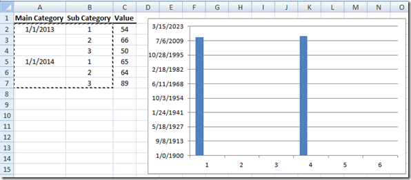
Fixing Your Excel Chart When the Multi-Level Category Label Option is Missing. - Excel Dashboard ...
Change axis labels in a chart - support.microsoft.com Right-click the category labels you want to change, and click Select Data. In the Horizontal (Category) Axis Labels box, click Edit. In the Axis label range box, enter the labels you want to use, separated by commas. For example, type Quarter 1,Quarter 2,Quarter 3,Quarter 4. Change the format of text and numbers in labels
Add a label and other information to axes in a Graph or Chart in Excel by Excel Made Easy
How to Add Data Labels in Excel - Excelchat | Excelchat After inserting a chart in Excel 2010 and earlier versions we need to do the followings to add data labels to the chart; Click inside the chart area to display the Chart Tools. Figure 2. Chart Tools. Click on Layout tab of the Chart Tools. In Labels group, click on Data Labels and select the position to add labels to the chart.
Fixing Your Excel Chart When the Multi-Level Category Label Option is Missing. - Excel Dashboard ...
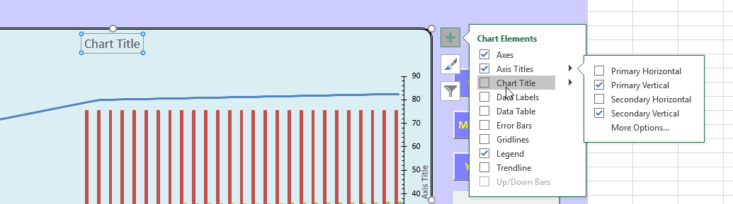
› documents › excelHow to add or move data labels in Excel chart? In Excel 2013 or 2016. 1. Click the chart to show the Chart Elements button . 2. Then click the Chart Elements, and check Data Labels, then you can click the arrow to choose an option about the data labels in the sub menu. See screenshot: In Excel 2010 or 2007. 1. click on the chart to show the Layout tab in the Chart Tools group. See ...

How to select best Excel Charts for Data Analysis & Reporting
How to Insert Axis Labels In An Excel Chart | Excelchat How to add vertical axis labels in Excel 2016/2013. We will again click on the chart to turn on the Chart Design tab . We will go to Chart Design and select Add Chart Element; Figure 6 – Insert axis labels in Excel . In the drop-down menu, we will click on Axis Titles, and subsequently, select Primary vertical . Figure 7 – Edit vertical axis labels in Excel. Now, we can enter the …
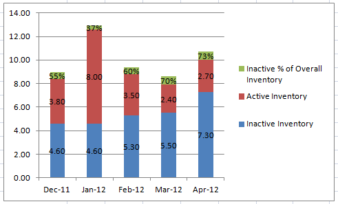
How-to Put Percentage Labels on Top of a Stacked Column Chart - Excel Dashboard Templates
How To Add Axis Labels In Excel [Step-By-Step Tutorial] First off, you have to click the chart and click the plus (+) icon on the upper-right side. Then, check the tickbox for 'Axis Titles'. If you would only like to add a title/label for one axis (horizontal or vertical), click the right arrow beside 'Axis Titles' and select which axis you would like to add a title/label. Editing the Axis Titles
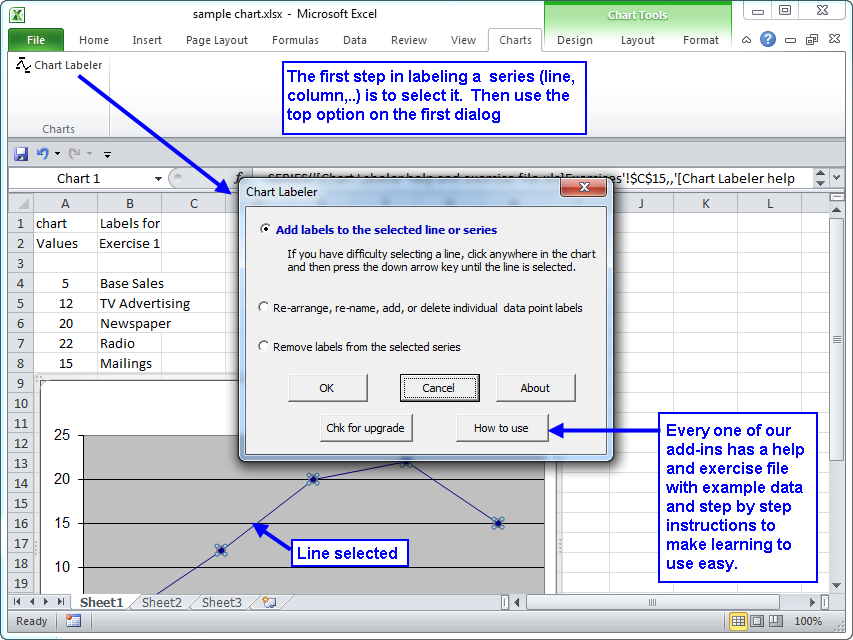
Chart Labeler for Microsoft Excel
How to Add Data Labels to an Excel 2010 Chart - dummies Use the following steps to add data labels to series in a chart: Click anywhere on the chart that you want to modify. On the Chart Tools Layout tab, click the Data Labels button in the Labels group. A menu of data label placement options appears: None: The default choice; it means you don't want to display data labels.

Pie Chart - PK: An Excel Expert
Unable to see the Label Position in excel chart ... Additionally, I found a workaround for it. You can set the position of a label first, then click Label Options > Data Label Series > Clone Current Label to quickly apply custom data label formatting to the other data points in the series. Best regards, Jazlyn. -----------------------. * Beware of scammers posting fake support numbers here.

How-to Use Data Labels from a Range in an Excel Chart - Excel Dashboard Templates
Change the format of data labels in a chart To get there, after adding your data labels, select the data label to format, and then click Chart Elements > Data Labels > More Options. To go to the appropriate area, click one of the four icons ( Fill & Line, Effects, Size & Properties ( Layout & Properties in Outlook or Word), or Label Options) shown here.

How to insert data labels to a Pie chart in Excel 2013 - YouTube
› solutions › excel-chatHow to Insert Axis Labels In An Excel Chart | Excelchat How to add vertical axis labels in Excel 2016/2013. We will again click on the chart to turn on the Chart Design tab . We will go to Chart Design and select Add Chart Element; Figure 6 – Insert axis labels in Excel . In the drop-down menu, we will click on Axis Titles, and subsequently, select Primary vertical . Figure 7 – Edit vertical axis labels in Excel. Now, we can enter the name we want for the primary vertical axis label. Figure 8 – How to edit axis labels in Excel

34 Label Chart In Excel - Labels Database 2020
How to hide zero data labels in chart in Excel? If you want to hide zero data labels in chart, please do as follow: 1. Right click at one of the data labels, and select Format Data Labels from the context menu. See screenshot: 2. In the Format Data Labels dialog, Click Number in left pane, then select Custom from the Category list box, and type #"" into the Format Code text box, and click Add button to add it to Type list box.

Charting in Excel - Adding Data Labels - YouTube
How to Create a Bar Chart With Labels Above Bars in Excel In the chart, right-click the Series “Dummy” Data Labels and then, on the short-cut menu, click Format Data Labels. 15. In the Format Data Labels pane, under Label Options selected, set the Label Position to Inside End. 16. Next, while the labels are still selected, click on Text Options, and then click on the Textbox icon. 17.

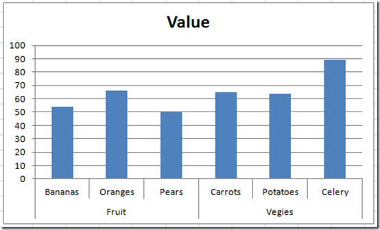
How to Create Multi-Category Chart in Excel - Excel Board
support.microsoft.com › en-us › officeEdit titles or data labels in a chart On a chart, click the label that you want to link to a corresponding worksheet cell. On the worksheet, click in the formula bar, and then type an equal sign (=). Select the worksheet cell that contains the data or text that you want to display in your chart. You can also type the reference to the worksheet cell in the formula bar.
Creating a chart with dynamic labels - Microsoft Excel 2013
Dynamically Label Excel Chart Series Lines • My Online ... Step 1: Duplicate the Series. The first trick here is that we have 2 series for each region; one for the line and one for the label, as you can see in the table below: Select columns B:J and insert a line chart (do not include column A). To modify the axis so the Year and Month labels are nested; right-click the chart > Select Data > Edit the ...

Cumulative Histogram
How to Add Axis Labels to a Chart in Excel | CustomGuide Add Data Labels. Use data labels to label the values of individual chart elements. Select the chart. Click the Chart Elements button. Click the Data Labels check box. In the Chart Elements menu, click the Data Labels list arrow to change the position of the data labels.

Excel Custom Chart Labels • My Online Training Hub
Edit titles or data labels in a chart Select the worksheet cell that contains the data or text that you want to display in your chart. You can also type the reference to the worksheet cell in the formula bar. Include an equal sign, the sheet name, followed by an exclamation point; for example, =Sheet1!F2 Press ENTER. Top of Page Reestablish the link for a data label

How to Visualize Age/Sex Patterns with Population Pyramids | Depict Data Studio
How to Place Labels Directly Through Your Line Graph in ... Right-click on top of one of those circular data points. You'll see a pop-up window. Click on Add Data Labels. Your unformatted labels will appear to the right of each data point: Click just once on any of those data labels. You'll see little squares around each data point. Then, right-click on any of those data labels.
Post a Comment for "42 how to show labels in excel chart"